On this page you can learn more about:
- Stochastic Error Identification and Modeling
- Linear and Nonlinear Filtering
- Bayesian Filtering
- Multi-Sensor Data Fusion
Stochastic Error Identification and Modeling
All sensor, model and observation errors in an integrated navigation system must be properly characterized in order to tune the underlying navigation filter.
Any error source can be described as superposition of bias- and noise-like components. The noise-like parts are a combination of different colors of noise, as there are brown, pink, white, blue and violet noise. To identify the noise in a sensor, e.g. an inertial gyro, a long-time recording is performed. The initial temperature effects have to be considered herein.
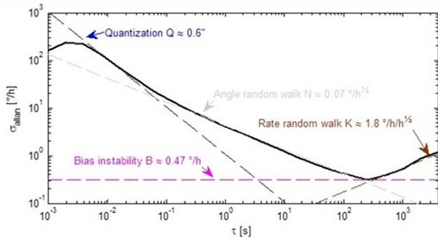
For the recorded sensor data are evaluation using either a power spectral density (PSD), Allan or Hadamard variance. From these typical sensor specification values can be evaluated. Furthermore low-fidelity stochastic sensor error models can be identified for the purpose of navigation filter tuning. High-fidelity stochastic sensor error modelling is performed to be used in simulation environments.
The noise-like sensor, model and observation errors are required to describe the time- and cross-correlation of the navigation solution. Obviously just bias-like sensor, model and observation errors can be estimated, of observable, in a navigation filter.
Literature
- IEEE standard specification format guide and test procedure for single-axis interferometric fiber optic gyros, Std. 952, 2008.
- A. Papoulis and S. U. Pillai, Probability, random variables, and stochastic processes, 4th ed. Boston, Mass.: McGraw-Hill, 2002.
- D. W. Allan, “Statistics of atomic frequency standards,” Proceedings of the IEEE, vol. 70, no. 3, pp. 221–230, 1965.
- M. S. Keshner, “1/f Noise,” Proceedings of the IEEE, vol. 70, no. 3, pp. 212–218, 1982.
- D. Simon, Optimal state estimation: Kalman, H-infinity and nonlinear approaches. Hoboken, N.J.: Wiley-Interscience, 2006.
Linear and Nonlinear Filtering
Optimal filtering is real-time capable data fusion fulfilling a mathematical optimality criterion. Rudolf E. Kálmán invented a set of equations for the propagation and correction of the filter state vector and corresponding covariance matrix of a dynamic system.
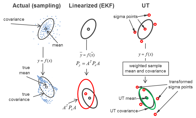
In the so-called Extended Kalman Filter (EKF) the state vector propagation and correction is carried out applying the nonlinear dynamic system, whereas the state covariance matrix propagation and correction are, as in the Conventional Kalman Filter (CKF), based on the linearized dynamic system. The optimality criterion used is the minimum of the trace of the state covariance matrix for the sake of simplicity of the resulting (Kalman) filtering equations.
The assumption of linear state covariance propagation and correction holds if and only if the nonlinearity and the initialization, state, sensor, model and observation errors are limited. When the limits are exceeded a nonlinear filtering approach is required. Particle filtering approaches transform a large number of particles from the domain of definition into the image range, where its covariance is estimated. Some years ago the so-called Unscented Transformation (UT) was invented, where for a n-dimensional state vector just 2n+1 sigma points are transformed by the unscented transform and the covariance is recovered in the image range only using these sigma points. This sometimes Unscented Kalman Filter (UKF) called approach is of second order accuracy in the state covariance propagation and correction. For the same accuracy order the Gaussian filter would not just require the Jacobian, but also the Hessian of the non-autonomous nonlinear ordinary differential equations of motion.
When the navigation dynamics of the platform under investigation is larger than the error dynamics, the error state space formulation shall be preferred.
Literature
- Seminar “Navigation and Data Fusion”.
- D. L. Hall and J. Llinas, Handbook of multisensor data fusion. Boca Raton, FL: CRC Press, 2001.
- S. J. Julier and J. K. Uhlmann, “A New Extension of the Kalman Filter to Nonlinear Systems,” in Proceedings Of AeroSense: The 11th Int. Symp. On Aerospace/Defense Sensing, Simulation and Controls: 1997.
- V. Krebs, Nichtlineare Filterung. München: Oldenbourg, 1980.
- C. T. Leondes, Theory and applications of Kalman filtering. Neuilly-sur-Seine: North Atlantic Treaty Organization, Advisory Group for Aerospace Research and Development, 1970.
- G. Minkler and J. Minkler, Theory and application of Kalman filtering. Palm Bay, Fla.: Magellan Book, 1993.
- A. H. Sayed, Fundamentals of adaptive filtering. New York, Hoboken, NJ: IEEE Press; Wiley, 2003.
- H. W. Sorenson, Kalman filtering: Theory and application. New York: IEEE Press, 1985.
- E. A. Wan and R. van der Merwe, “The Unscented Kalman Filter for Nonlinear Estimation,” in Proceedings of the IEEE Symposium: AS-SPCC, 2000.
Bayesian Filtering
Recursive estimators are mostly based on the Bayes’ theorem:
![]()
The Bayes’ theorem describes how the knowledge of the system state is combined with measurement information to get a better estimate of the state. The knowledge of the system state is given with the “a priori” probability of the state Pr(X), which initially is mostly a “good guess”. The measurement information is the likelihood probability Pr(Y|X). The likelihood of a measurement is thereby depending on the state. The likelihood and the “a priori” probability are multiplied and normalized through the evidence Pr(Y), which is a normalization factor. The resulting new probability of the state is known as the “a posteriori”.
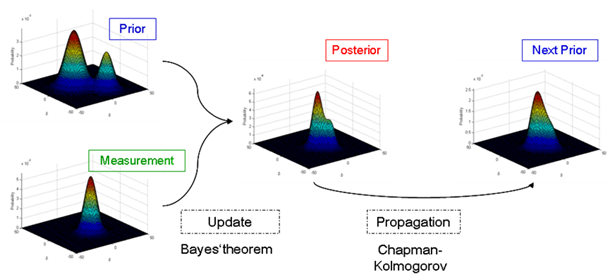
The probabilities could in general be described by probability density functions, which can be discretized as grid or particle methods. In the linear case the Gaussian distribution is mostly used due to the fact, that a Gaussian distribution for both the “a priori” and the likelihood probability lead again to a Gaussian “a posteriori” (conjugate distribution property), therefore the kind of distributions are not changing in the recursive process. The Kalman filter is a good example for a linear Bayesian estimator. When the Gaussian property is not fulfilled in some sufficient approximation for all phases of the application under consideration, nonlinear Bayesian filtering is required.
The state estimate can either be the state with the highest probability (maximum “a posteriori” estimator) or the mean state resulting in the minimum mean square estimator. When the next measurement is processed the former “a posteriori” state probability is the new “a priori” probability.
Literature
- Särkkä, Bayesian filtering and smoothing. Cambridge, U.K, New York: Cambridge University Press, 2013.
- V. Candy, Bayesian signal processing: Classical, unscented and particle filtering methods. Oxford: Wiley-Blackwell, 2009.
- Ristic and S. Arulampalam, Beyond the Kalman filter: Particle filters for tracking applications. Boston, MA: Artech House, 2004.
- Chen, Bayesian Filtering: From Kalman Filters to Particle Filters, and Beyond. Available: http://www.dsi.unifi.it/users/chisci/idfric/Nonlinear_filtering_Chen.pdf.
Multi-Sensor Data Fusion
Multi-sensor multi-frequency data fusion requires more than just filtering theory.
Each sensor must be synchronized with respect to a central clock to keep track on time of validity of the measurement, time of transmission of the quantity and time of data fusion. Whereas a sensor measurement is done periodically with just a very small time jitter a navigation subsystem observation may due to computational variations get available in a much more irregular manner. Especially through these computational variations it could happen, that older navigation data gets available after newer navigation data already has been processed. These effects are called out-of-sequence-measurements and can be treated algorithmically.
Before navigation data from different sources can be fused they also must refer to the same point in space. Thus large lever arm compensations are commonly performed and, if necessary, subsystem frames aligned.
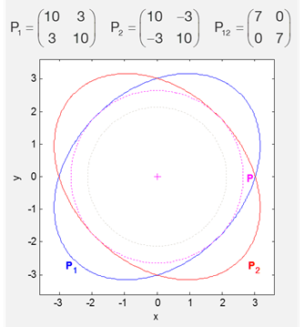
Plausibility tests aim to avoid interface problems and statistical tests care for integrity issues. Since navigation sensors and subsystems have in general already been integrated in the past, new measurements or observations cannot be assumed to be uncorrelated. An increase of measurement or observation rates scales the computational effort, but may not provide an equivalent amount of information. The stronger the correlation becomes the less improvement can be expected.
Literature
- Seminar “Navigation and Data Fusion”.
- D. L. Hall and J. Llinas, Handbook of multisensor data fusion. Boca Raton, FL: CRC Press, 2001.
| ⇦ Navigation Aids | return to overview | Navigation Systems ⇨ |